2. First Steps

In this session we will introduce the most fundamental aspects of using R, and at the end of the session you should feel more comfortable engaging with the many online resources that are out there to help people learn R to analyse data.

You should come away from this tutorial with a general sense of meaning for the following terms:

data types - data structures - objects - functions - arguments - object classes - assignment - operators - dataframes - pipes - packages - CRAN

First steps

Learning anything from scratch requires starting somewhere. So let’s start here:

# You can play along by typing this code into your own console
  x <- c(1, 2, 3)
  x

[1] 1 2 3

Working from right to left, there are three key elements in the code above.

The first is the function c(). A function in R is like a function in math. It is something that takes one or more inputs and converts them into an output. In this example, the function c() creates a vector containing the three numbers 1, 2, 3.

The next element is the assignment operator <-, and the final one is x, which is an object we’ve now created, using <- , that contains the results of the function c(1, 2, 3).

At it’s most basic, R scripting is just repeating this process, using the right functions on the relevant input objects to create new, useful output oubjects.

output <- function(inputs)

It’s really just that simple. The hardest part is learning over time what functions you should use for which tasks.

As aside on assignment

Other programming languages use = as an assignment operator and technically you can use it in R as well, though people have written many words about why you shouldn’t.

  x = c(1, 2, 3)      
  x

[1] 1 2 3

The assignment operator <- can also be used as -> though you will only rarely see this in practice.

  c(1, 2, 3) -> x      
  x

[1] 1 2 3

Data types, structures, and object classes

In the example above, we took three pieces of data, all of which were numbers, and grouped them together as a vector. A numeric vector, if you will.

  class(x)

[1] "numeric"

  typeof(x)

[1] "double"

In this example, numeric refers to the class of the object, while a vector is the most primitive data structure in R ¹. It is essentially a list of n elements that are all of the same type, where type is a description of how the data are stored in memory (and “double” means double-precision floating-point format which is a common way to store decimal numbers).

We don’t want to get too deep in the weeds here, but because there is a close correspondence between class and type, the important thing to understand more generally is that the class of an object can influence the behavior of functions we might use on said object. We will come back to this idea shortly.

Of course data comes in forms other than numbers. For example, maybe we are working with character data (also known as sting or text data).

  y <- c("Kareem", "MJ", "Lebron")
  class(y)

[1] "character"

  typeof(y)

[1] "character"

And the other two important types of data are logical and integer values ².

  logicals <- c(TRUE, TRUE, FALSE)
  class(logicals)

[1] "logical"

  typeof(logicals)

[1] "logical"

To create a vector of integers, we have to explicitly tell R we want integers, and not decimal numbers.

  integers <- c(as.integer(1), as.integer(2), as.integer(3)) 
  integers <- as.integer(c(1, 2, 3))       
  # The two lines above are equivalent
  class(integers)

[1] "integer"

  typeof(integers)

[1] "integer"

Critically, if we try to combine different data types in the same vector, R will convert all the elements as needed to remove the conflict.

  z <- c(x, y) # Combine the x and y vectors into a single vector, z
  z

[1] "1"      "2"      "3"      "Kareem" "MJ"     "Lebron"

  class(z)

[1] "character"

  typeof(z)

[1] "character"

In the example above, combining numbers and characters into the vector turned everything into character data since characters can’t possibly be numbers, and hence the "" now surrounding the numbers. Similarly, if we combine integers and decimal numbers in a vector, R will force them all to be stored as decimal numbers, since converting decimal numbers to integers could result in information loss.

  mix <- c(integers, x)
  mix

[1] 1 2 3 1 2 3

  class(x)

[1] "numeric"

  typeof(x)

[1] "double"

I also want to introduce integer type data that are associated with character labels. We call these factor data and they are very useful – so much so that we will come back to them in a separate tutorial later.

  y

[1] "Kareem" "MJ"     "Lebron"

  class(y) # y starts as a character vector

[1] "character"

  # An error, because we can't turn text into a number:
  as.numeric(y) 

Warning: NAs introduced by coercion

[1] NA NA NA

  # We can create a factor vector like this:
  y_factor <- factor(y) 
  y_factor # This displays the labels (called levels)

[1] Kareem MJ     Lebron
Levels: Kareem Lebron MJ

  # Not an error because a factor is a labelled integer:
  as.numeric(y_factor) 

[1] 1 3 2

  class(y_factor)

[1] "factor"

  typeof(y_factor)

[1] "integer"

  levels(y_factor)

[1] "Kareem" "Lebron" "MJ"    

And finally we have dates, which are numeric data that are presented in a date format. Again, working with dates will recieve special treatment later.

  dates <- c("2025-12-12", "2025-12-13")
  dates

[1] "2025-12-12" "2025-12-13"

  typeof(dates)

[1] "character"

  dates <- as.Date(dates)
  dates

[1] "2025-12-12" "2025-12-13"

  typeof(dates) 

[1] "double"

  class(dates)

[1] "Date"

  c(dates, y) # Tries to convert characters to date but can't

Error in `charToDate()`:
! character string is not in a standard unambiguous format

  c(dates, x) # Does manage to convert numbers to dates...

[1] "2025-12-12" "2025-12-13" "1970-01-02" "1970-01-03" "1970-01-04"

  as.numeric(c(dates, x))

[1] 20434 20435     1     2     3

  # Because dates are the number of days before/since Jan 1, 1970
  as.Date(0)

[1] "1970-01-01"

Data frames

While vectors are an incredibly exciting data structure, they can only take us so far. Ultimately we want to work with datasets, and as we all know, datasets are two-dimensional matrices that contain variables (or fields) in the columns that characterize the observations in the rows.

R has matrix (two dimensions) and array (more than two dimensions) data structures, but like vectors, they can only contain a single type of data, and that’s not going to get us very far towards the types of datasets we use in medicine and health research.

  a_matrix_woah <- matrix(1:10, nrow = 2)
  a_matrix_woah

     [,1] [,2] [,3] [,4] [,5]
[1,]    1    3    5    7    9
[2,]    2    4    6    8   10

  class(a_matrix_woah)

[1] "matrix" "array" 

  dim(a_matrix_woah) # Dimensions (n rows, n columns)

[1] 2 5

R also has a list data structure, which is basically a 1D vector but that can contain different types of data.

  a_list <- list(1, 2, "Kareem", "MJ")
  class(a_list)

[1] "list"

Lists in R can actually contain just about anything, including entire vectors and other objects, making them very useful.

# A list of other objects we've created
  big_list <- list(1:14, x, y, z, a_matrix_woah) 
  big_list

[[1]]
 [1]  1  2  3  4  5  6  7  8  9 10 11 12 13 14

[[2]]
[1] 1 2 3

[[3]]
[1] "Kareem" "MJ"     "Lebron"

[[4]]
[1] "1"      "2"      "3"      "Kareem" "MJ"     "Lebron"

[[5]]
     [,1] [,2] [,3] [,4] [,5]
[1,]    1    3    5    7    9
[2,]    2    4    6    8   10

And this brings us to the most important data structure in R, the data.frame.

On a technical level, a data.frame in R is a named list containing vectors. While each vector can only contain one type of data (because they are vectors), a data.frame can contain vectors of different types (because it’s a list). Importantly, the vectors in a data.frame much all have the same number of elements (or lengths), and all the vectors must have a name.

# Our first data.frame can you feel the excitement?

  data <- data.frame(rank = x, player = y)
  data

  rank player
1    1 Kareem
2    2     MJ
3    3 Lebron

  class(data)

[1] "data.frame"

  names(data)

[1] "rank"   "player"

  dim(data)

[1] 3 2

Selection

In the examples above, we created objects that we can think of as being made up of other, “smaller” objects. For example, the numeric vector x <- c(1, 2, 3) contains three numbers each of which we can think of as three separate vectors of length 1.

We often want to extract bits of information from larger objects, and the main way to do this is through selection using brackets [ ] . For example, if I want to the first element of a one dimensional vector, I can do this:

  x <- c(1, 2, 3)
  x

[1] 1 2 3

  x[1]

[1] 1

For a two-dimensional object like our data.frame, I can do this:

  data

  rank player
1    1 Kareem
2    2     MJ
3    3 Lebron

  data[1, 2] # Remember, it's always Row and then Column. RC

[1] "Kareem"

Lists are a little more complicated. The best analogy I’ve come across is that they are like a train composed of train cars. If we use [] to select elements of a list, we get a list object of length 1 with it’s contents.

  big_list[1] # Select the first train car

[[1]]
 [1]  1  2  3  4  5  6  7  8  9 10 11 12 13 14

  class(big_list[1]) # List

[1] "list"

However, if you want to fully extract whatever is inside the train car, we need to use double brackets [[ ]].

  big_list[[1]] # Select whatever is *inside* the first train car

 [1]  1  2  3  4  5  6  7  8  9 10 11 12 13 14

  class(big_list[[1]]) # Vector

[1] "integer"

These rules are important since data.frames are also lists, and because the behavior of functions can be influenced by the class of the objects they are acting on (as I mentioned above).

  class(data[[1]]) # Vector

[1] "numeric"

  class(data[1])   # Data.frame

[1] "data.frame"

A final point relevant to dataframes (and named lists more generally) is the $ operator, which is equivalent to [[]] but that uses the name of the column rather than the index.

  data[[1]]

[1] 1 2 3

  class(data[[1]]) # Numeric vector

[1] "numeric"

  data$rank

[1] 1 2 3

  class(data$rank) # Numeric vector

[1] "numeric"

  data$rank[1] # First element of the vector

[1] 1

In the examples above, we’ve used selection to extract elements from an object, but we can also use “overwrite” elements in the same way. You will do this a lot, unless you are only ever in receipt of perfect data :)

  x

[1] 1 2 3

  x[1] <- 99
  x

[1] 99  2  3

Functions and packages

I have spent many years using and teaching R. Whenever you are having a problem with R that just doesn’t make sense, experience says that it will often come down to one of two problems:

• There is a typo in your code. Look again. And again. It’s there. I promise.

• If it’s not a typo, then the class of the object you applying a function to won’t allow the function to do what you want it to do. This is to say that functions can be sensitive to object class.

For example, the function mean works on numeric vectors.

# This doesn't work because data[1] is a dataframe
  class(data[1])

[1] "data.frame"

  mean(data[1])  

Warning in mean.default(data[1]): argument is not numeric or logical: returning
NA

[1] NA

# This works because data[[1]] is a vector
  class(data[[1]])

[1] "numeric"

  mean(data[[1]])

[1] 2

The behavior of functions is also controlled by its arguments. For example, consider the following two matrices.

  matrix_1 <- matrix(c(1:10), nrow = 2)
  matrix_1

     [,1] [,2] [,3] [,4] [,5]
[1,]    1    3    5    7    9
[2,]    2    4    6    8   10

  matrix_2 <- matrix(c(1:10), nrow = 5)
  matrix_2

     [,1] [,2]
[1,]    1    6
[2,]    2    7
[3,]    3    8
[4,]    4    9
[5,]    5   10

In that example, nrow is an argument of the function matrix that set the number of rows for the resulting matrix.

The order of arguments in a function matters in that you don’t technically need to name them as long as you use them in the right order. For example, the following will work just fine without the nrow.

  matrix(c(1:10), 5) 

     [,1] [,2]
[1,]    1    6
[2,]    2    7
[3,]    3    8
[4,]    4    9
[5,]    5   10

Or you can use the arguments out of order, but only if you name them.

  matrix(nrow = 5, data = c(1:10)) 

     [,1] [,2]
[1,]    1    6
[2,]    2    7
[3,]    3    8
[4,]    4    9
[5,]    5   10

And many arguments have defaults. For example, the default for matrix is nrow = 1.

  matrix(data = c(1:10)) # Assumes you want nrow = 1

      [,1]
 [1,]    1
 [2,]    2
 [3,]    3
 [4,]    4
 [5,]    5
 [6,]    6
 [7,]    7
 [8,]    8
 [9,]    9
[10,]   10

So how can you possibly know all of this about a particular function? Thankfully R has a built in help function. To learn about a function you just type in ?function_name and a window with information about that function will open. So in your own console, type ?mean and read what pops up in the help tab in your RStudio view.

Pipes

You will regularly need for than one function to accomplish your goals. There are basically three ways you might code the use of multiple functions, one of which involves the pipe operator, |>.

Let’s say we want to take the mean of some set of numbers and then round the result to 1 decimal place. Here are at least three ways to code this:

# Option 1   
  x <- c(1, 43, 4019, 4)    
  x <- mean(x)   
  x <- round(x, 1)   
  x    

[1] 1016.8

# Option 2: Nesting functions   
  x <- round(mean(c(1, 43, 4019, 4)), 1)    
  x    

[1] 1016.8

# Option 3: Using pipes     
  x <- c(1, 43, 4019, 4) |> mean() |> round(1)   
  x 

[1] 1016.8

As you can see, the basic function of the pipe |> is to take what’s on the left and use it as the first argument in the function on the right. How you choose to write your code is entirely up to you. My own work tends to be a mix of all three options, though generally I try to avoid nesting because I find it more challenging to read and thus to spot errors in.

Packages and CRAN

R is an open source programming language with a vibrant community of users and developers. This community, over many years, has collectively written many thousands of packages. The vast majority of those packages can be described as collections of functions, as well as perhaps example data.frames. So a big part of using R is to identify and then accesss the package(s) that contain the function(s) you need to conduct the analysis you want to conduct.

An important place to find useful R packages are the CRAN Task Views. These are basically curated lists of packages organized by area.

So where do you get packages? For now the answer is that you get them from CRAN and its repository of contributed packages. Thankfully, access to CRAN is basically built into RStudio, so if you want to install a package, you use the install.packages function. In the next tutorial, we are going to introduce ggplot for data visualization, so let’s install that package now by pasting this into your console: install.packages("ggplot2").

When you want to actually load the package, you take it out of the “library”.

  library(ggplot2)

And now you have access to the package contents in your environment, including the function ggplot().

  data |>
  ggplot(aes(x = player, y = rank)) +
    geom_point()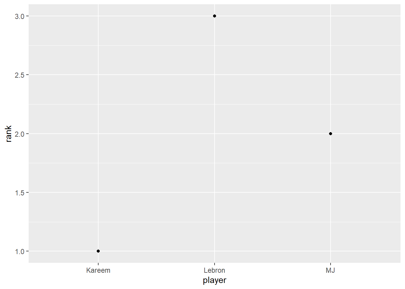

Summary

Click the links below to review key terms as explained in Hands-On Programming with R by Garrett Grolemund.

data types

data structures

selection

objects

functions

object classes

dataframes

packages

Footnotes

1. For those coming from other programming languages, there are technically no scalars in R, just vectors of length 1. But I’m not a programmer and have no idea why anyone would care about this, so will leave it at that :)

2. There are also complex and raw types, but I’ve never used either and don’t suspect you will need to either.